White papers

Use our white paper search or select a quick entry below to display white papers based on product type, supplier or application.

The 10 latest white papers
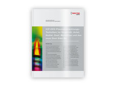
Comparing ICP-OES Analyzers' Plasma Views: Axial, Radial, Dual, MultiView, and Dual Side-On
A Comparison of the Basic Functioning of the Technologies
View white paper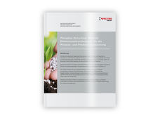
Effluent Phosphate Recovery & Recycling
The Latest Analytical Solutions
View white paper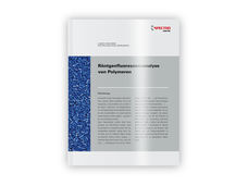
X--ray Fluorescence Analysis of Polymers
Advanced elemental analysis offers exceptional possibilities and advantages
View white paper

White papers by application


White papers by product type

Get the chemical industry in your inbox
From now on, don't miss a thing: Our newsletter for the chemical industry, analytics, lab technology and process engineering brings you up to date every Tuesday and Thursday. The latest industry news, product highlights and innovations - compact and easy to understand in your inbox. Researched by us so you don't have to.
Promote your white papers on chemeurope.com
You spend a lot of time writing white papers and technical articles and offer them on your website. But the access figures are sobering. What can you do to make your white papers reach more interested parties?
On chemeurope.com, which has over 2.3 million users, your potential customers search specifically for white papers and technical articles that explain methods and explain applications.
You receive high-quality sales leads
You position your company as an expert in your field of expertise
Once written, your content generates sales leads again and again
Curious? Learn more now